The goal of bmggum is to estimate Multidimensional Generalized Graded Unfolding Model (MGGUM) using Bayesian method. Specifically,the R package rstan that utilizes the Hamiltonian Monte Carlo sampling algorithm was used for estimation. Below are some important features of the bmggum package:
You can install the development version of bmggum from GitHub:
devtools::install_github("Naidantu/bmggum")This is a basic example that shows you how to prepare data, fit the model, extract and plot results.
library(bmggum)

## basic example code
## Step 1: Input data
# 1.1 Response data in wide format
GGUM.Data <- c(1,4,4,1,1,1,1,1,1,1,4,1,1,3,1,1,NA,2,NA,3,2,2,2,1,3,2,NA,2,1,1,2,1,NA,NA,NA,1,3,NA,1,2)
GGUM.Data <- matrix(GGUM.Data,nrow = 10)

# 1.2 A two-row data matrix: the first row is the item number (1,2,3,4...); the second row indicates the signs of delta for each item (-1,0,1,...). For items that have negative deltas for sure, "-1" should be assigned; for items that have positive deltas, "1" should be assigned; for items whose deltas may be either positive or negative (e.g., intermediate items), "0" should assigned. We recommend at least two positive and two negative items per trait for better estimation.
delindex <- c(1,-1,2,1,3,-1,4,1)
delindex <- matrix(delindex,nrow = 2)

# 1.3 A row vector mapping each item to each trait. For example, c(1,1,1,2,2,2) means that the first 3 items belong to trait 1 and the last 3 items belong to trait 2.
ind <- c(1,1,2,2)
ind <- t(ind)

# 1.4 An p*c person covariate matrix where p equals sample size and c equals the number of covariates. The default is NULL, meaning no person covariate.
covariate <- c(0.70, -1.25, 0.48, -0.47, 0.86, 1.25, 1.17, -1.35, -0.84, -0.55)

## Step 2: Fit the MGGUM model
mod <- bmggum(GGUM.Data=GGUM.Data, delindex=delindex, trait=2, ind=ind, option=4, model="UM8", covariate=covariate)
#> [1] "Case 9 was deleted because they endorse the same response option across all items"

## Step 3: Extract the estimated results
# 3.1 Extract the theta estimates
theta <- extract(x=mod, pars='theta')
# Turn the theta estimates into p*trait matrix where p equals sample size and trait equals the number of latent traits
theta <- theta[,1]
# nrow=trait
theta <- matrix(theta, nrow=2)
theta <- t(theta)
# theta estimates in p*trait matrix format
theta
#>               [,1]        [,2]
#>  [1,]  1.000478918  0.03863573
#>  [2,] -1.517330074 -0.29803217
#>  [3,] -1.210468411 -0.60363516
#>  [4,]  0.685109657  1.00255476
#>  [5,]  0.085690711 -0.76981168
#>  [6,]  0.213125900 -0.85653665
#>  [7,]  0.879698855  0.23162129
#>  [8,]  0.009440613  0.49411920
#>  [9,]  0.642475444  0.85830443

# 3.2 Extract the tau estimates
tau <- extract(x=mod, pars='tau')
# Turn the tau estimates into I*(option-1) matrix where I equals the number of items and option equals the number of response options
tau <- tau[,1]
# nrow=option-1
tau <- matrix(tau, nrow=3)
tau <- t(tau)
# tau estimates in I*(option-1) matrix format
tau
#>            [,1]       [,2]      [,3]
#> [1,] -0.8439766 -1.5462686 -2.349370
#> [2,] -1.5469739 -1.8916896 -1.088957
#> [3,] -3.1834081 -0.8843948 -0.849958
#> [4,] -2.3538086 -1.3330377 -1.060610

# 3.3 Extract the lambda estimates
lambda <- extract(x=mod, pars='lambda')
# lambda[1,1] is the coefficient linking person covariate 1 to latent trait 1
# lambda[1,2] is the coefficient linking person covariate 1 to latent trait 2
lambda
#>                   mean    se_mean        sd       2.5%        50%     97.5%
#> lambda[1,1]  0.3036433 0.02287562 0.4925701 -0.5797526  0.2751898 1.3980741
#> lambda[1,2] -0.3277382 0.04226484 0.6855767 -2.0121720 -0.2743221 0.9248035
#>                n_eff     Rhat
#> lambda[1,1] 463.6499 1.006357
#> lambda[1,2] 263.1199 1.014433

## Step 4: Obtain model fit statistics
waic <- modfit(x=mod, index='waic')
loo <- modfit(mod)

## Step 5: Plottings
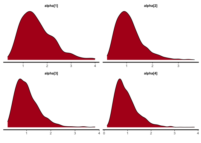
# 5.1 Obtain the density plots for alpha
bayesplot(x=mod, pars='alpha', plot='density', inc_warmup=FALSE)
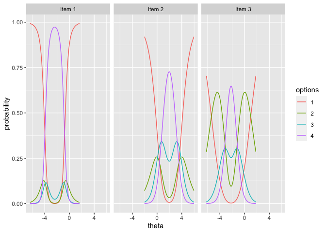
## Step 6: Plotting observable response categories (ORCs) for items
# 6.1 Obtain item plots with ORCs for item 1, 2, 3
itemplot(x=mod, items = 1:3)