

datacleanr is a flexible and efficient tool for
interactive data cleaning, and is inherently
interoperable, as it seamlessly integrates into
reproducible data analyses pipelines in
R.
It can deal with nested tabular, as well as spatial and time series data.
The latest release on CRAN can be installed using:
install.packages("datacleanr")You can install the development version of datacleanr
with:
remotes::install_github("the-hull/datacleanr")If you are using macOS, please make sure you have
XQuartz installed, especially if you’ve recently updated
your system. See these instructions here: https://CRAN.R-project.org/bin/macosx/
**In case the package installation fails due to a compilation error
from magick, please try installing the dev headers for
magick with
sudo apt-get install libmagick++-dev. Also see this gh
issue.
datacleanr is developed using the shiny package, and relies on
informative summaries, visual cues and interactive data selection and
annotation. All data-altering operations are documented, and converted
to valid R code (reproducible recipe),
that can be copied, sent to an active RStudio script, or
saved to disk.
There are four tabs in the app for these tasks:
R expression to
filter/subset data.dcr_app also returns all intermediate and
final outputs invisibly to the active R session for later
use (e.g. when batch processing)Note, maps require columns lon and lat (X
and Y) in decimal degrees in the data set to render.
TRUE\FALSE) column named
.dcrflag is present, corresponding observations are
rendered with different symbols in plots and maps. Use this feature to
validate or cross-check external quality control or outlier flagging
methods.# prepare data into species sub-sets
iris_split <- split(x = iris,
f = iris$Species)
# run for each species
dcr_iris <- lapply(iris_split,
function(split){
datacleanr::dcr_app(split)
})The documentation for (?dcr_app()) explains the basic
use and all features. Throughout the app, there are conveniently-placed
help links that provide details on features.
Launch datacleanr’s interactive app with
dcr_app(). The following examples demonstrate basic use and
highlight features across the four app tabs.
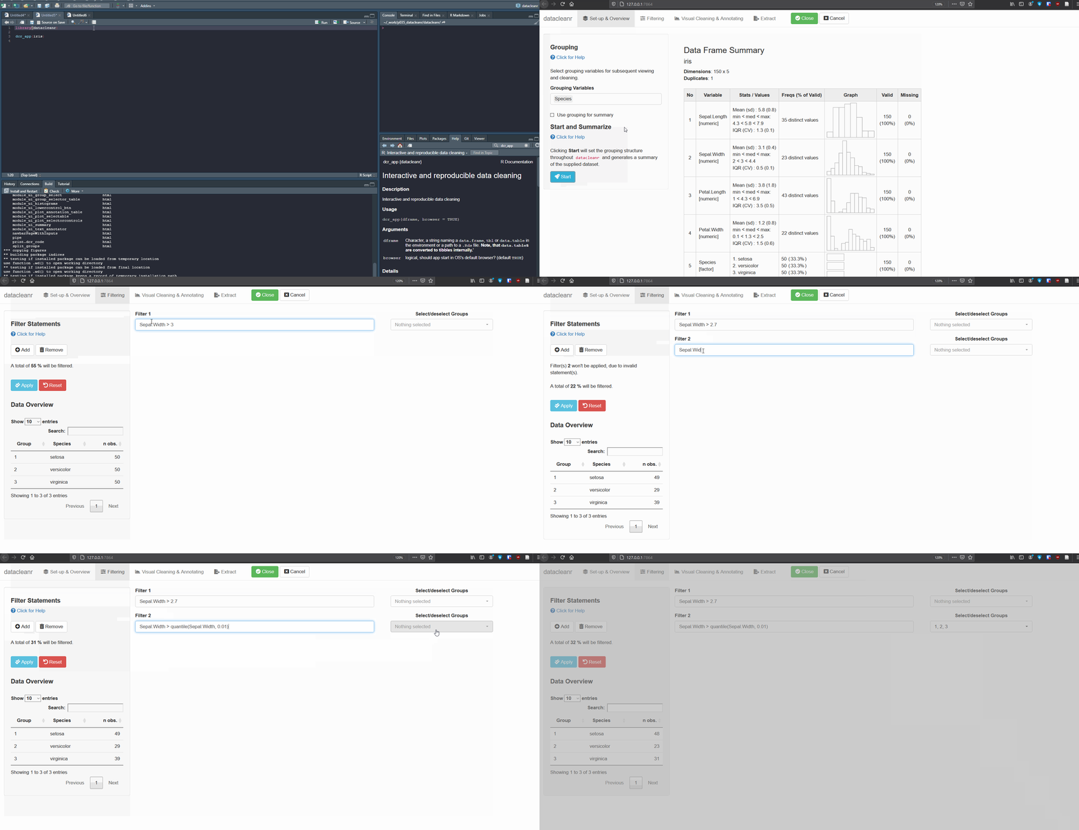
Define the grouping structure (used throughout app for scoping filters and plotting), and generate an informative overview.
library(datacleanr)

# group by species
dcr_app(iris)
Add/Remove filter statement boxes, and apply (valid) expressions -
either to the entire data set, or scoped to individual groups. Filtering
relies on R expressions passed to
dplyr::filter(), so, for example, valid statements for
iris are:
    Species == 'setosa'
    Species %in% c('setosa','versicolor')
    Sepal.Width > quantile(Sepal.Width, 0.05)
Any function returning a logical vector
(i.e. TRUE/FALSE), can be employed here!
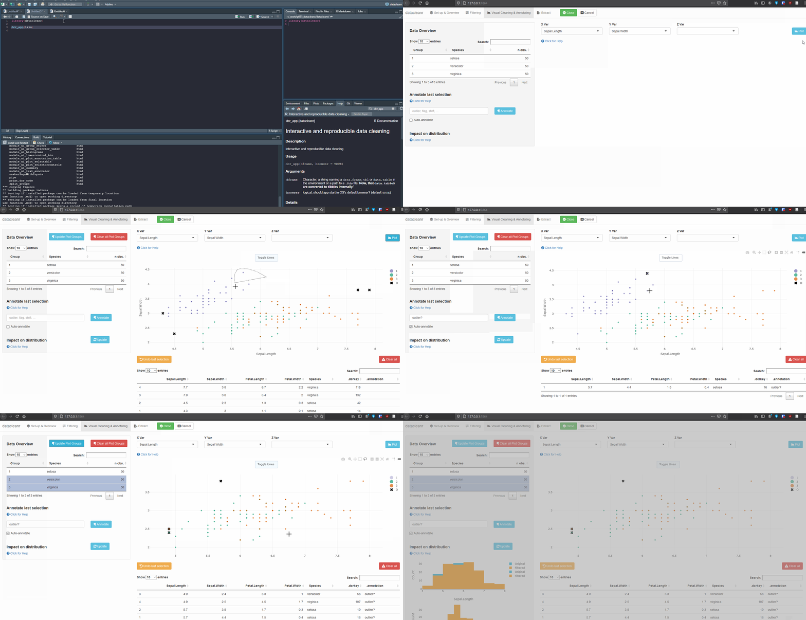
Interactive visualization allow seamless scrolling, panning and zooming to select and annotate individual observations (or sections with lasso/box select tool). Show and hide groups using the group selection table (left) or the legend (right).
.dcrflag to interface with external QA/QClibrary(datacleanr)
library(dplyr)
iris_mod <- iris %>%
group_by(Species) %>%
# .dcrflag provides additional visual cue in visualization tab
# based on TRUE/FALSE
mutate(.dcrflag = Sepal.Width < quantile(Sepal.Width, 0.05))
dcr_app(iris_mod)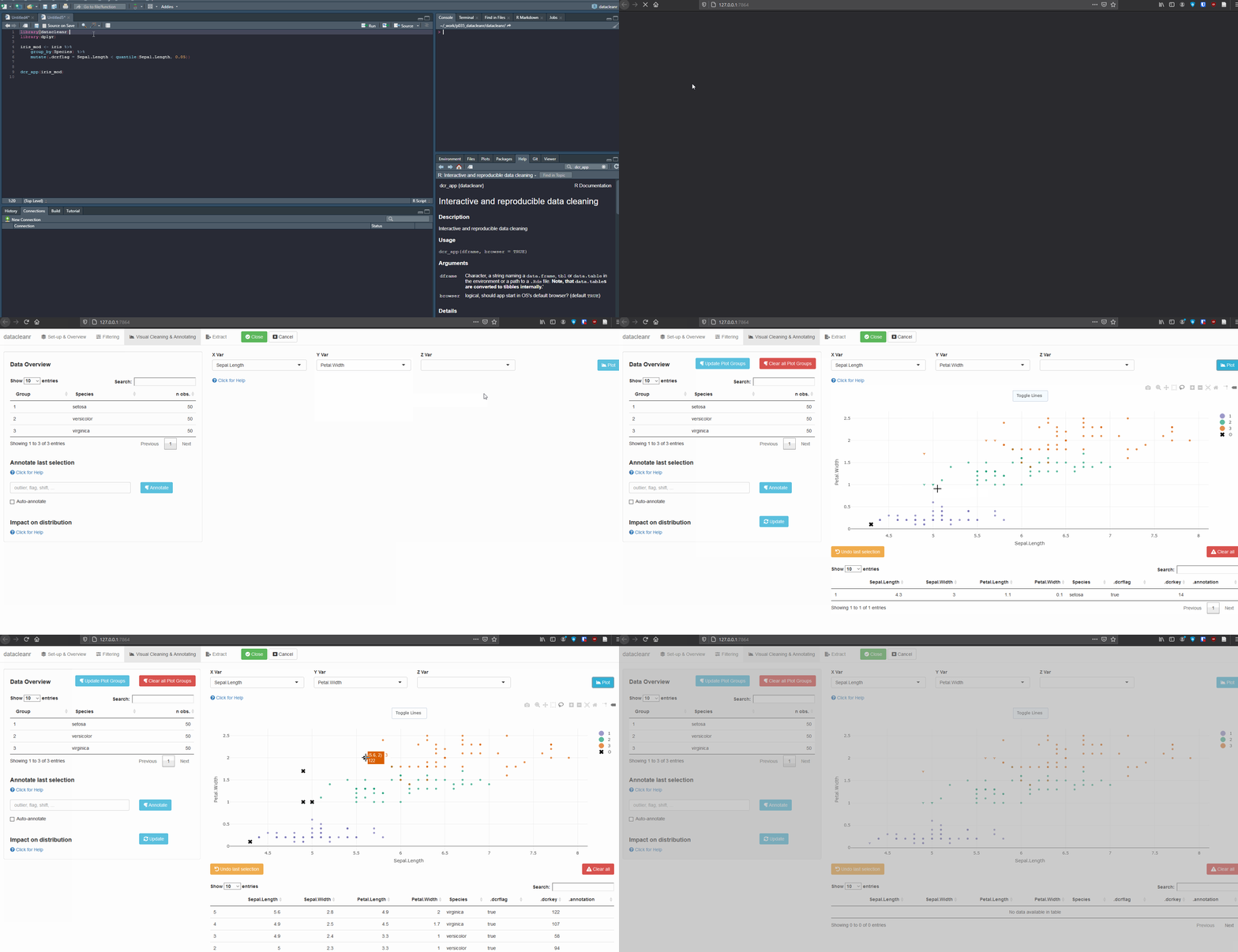
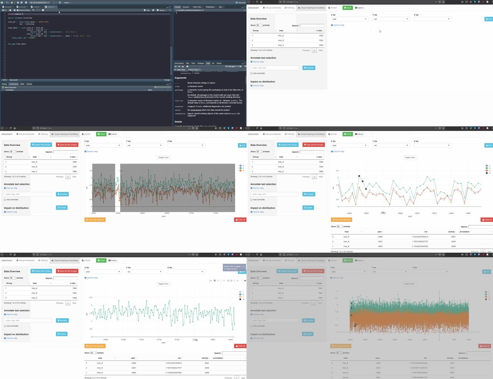
Any numeric or POSIXct column (in X or Y
dimension) can be used to visualize time series. Use the
Toggle Lines button above the plot to facilitate
exploration.
Example 1:
library(dplyr)

dplyr::glimpse(treering)
tree_df <- data.frame(year = -6000:1979,
           val = treering)

# make synthetic data
tree_data <- list(tree_A = tree_df,
                  tree_B = tree_df %>%
                      mutate(val = val + rnorm(nrow(.), 0.5, 0.2)),
                  tree_C = tree_df %>%
                      mutate(val = val + rnorm(nrow(.), mean = -0.03, 0.1))) %>%
    bind_rows(.id = "tree")

# group by tree and inspect
dcr_app(tree_data)
(Note, selections are arbitrary and for demonstration only)
Example 2:
No GIF
library(dplyr)
library(lubridate)
data("storms", package = "dplyr")

storms_mod <- storms %>%
    mutate(timestamp = lubridate::ymd_h(paste(year, month, day, hour)))

# Group by name (198 groups)
# Check "Emily"
dcr_app(storms_mod)Interactive maps rely on Mapbox
for plotting. Therefore, you will need to make an account, from which an
access token needs to be copied into your .Renviron
(e.g. MAPBOX_TOKEN=your_copied_token). A simple way to do
this is using the convenient usethis package to access the
file:
usethis::edit_r_environ()Select columns lon and lat for plotting to
get started.
Example 1
library(datacleanr)
library(dplyr)

airport_data <- read.csv('https://plotly-r.com/data-raw/airport_locations.csv') %>%
    rename(lon = long)

# group by state
dcr_app(airport_data)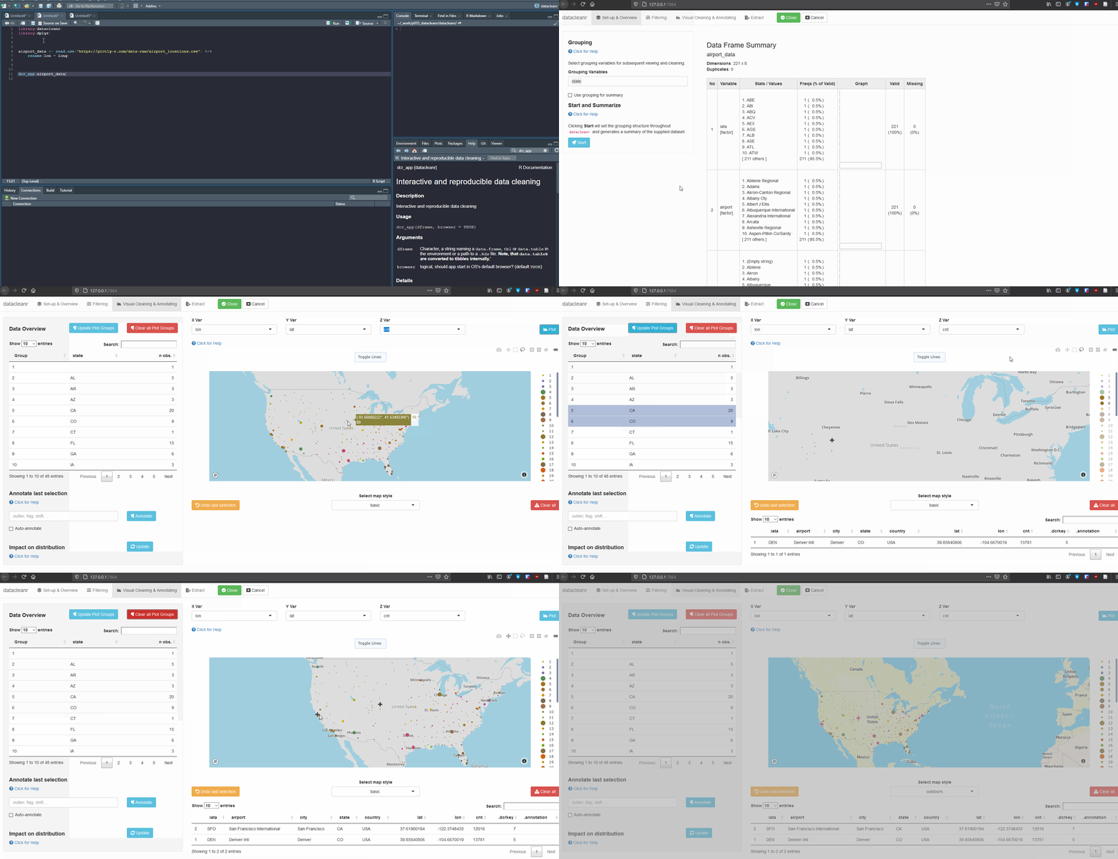
Example 2
No GIF
library(dplyr)
library(lubridate)
data("storms", package = "dplyr")


storms_mod <- storms %>%
    rename(lon = long)

# Group by name (198 groups)
# Check "Bonnie"
dcr_app(storms_mod)All grouping, filtering and selections/annotations are translated to
R code, which can be sent to an RStudio
script, copied to the clipboard, or - when dcr_app is
launched with a file path - save options are made available. For large
selections/annotations we recommend saving the script separately, and
sourcing it (i.e. source("your_datacleanr_script.R"))
during later analyses.
Caution: When selections / annotations are greater than ~
1000 points, it is recommended to use datacleanr with an
*.RDS file (see below). This is because the resulting
Reproducible Recipe (script) can slow down the RStudio IDE, if it has
more than a few thousand lines.The next version of
datacleanr will allow choosing between script-only recipes,
and the option with an the intermediate file for storing annotations.
Both approaches with their current implementation are shown shown
below.
Example 1
Launching with an object from R:
library(datacleanr)
dcr_app(iris)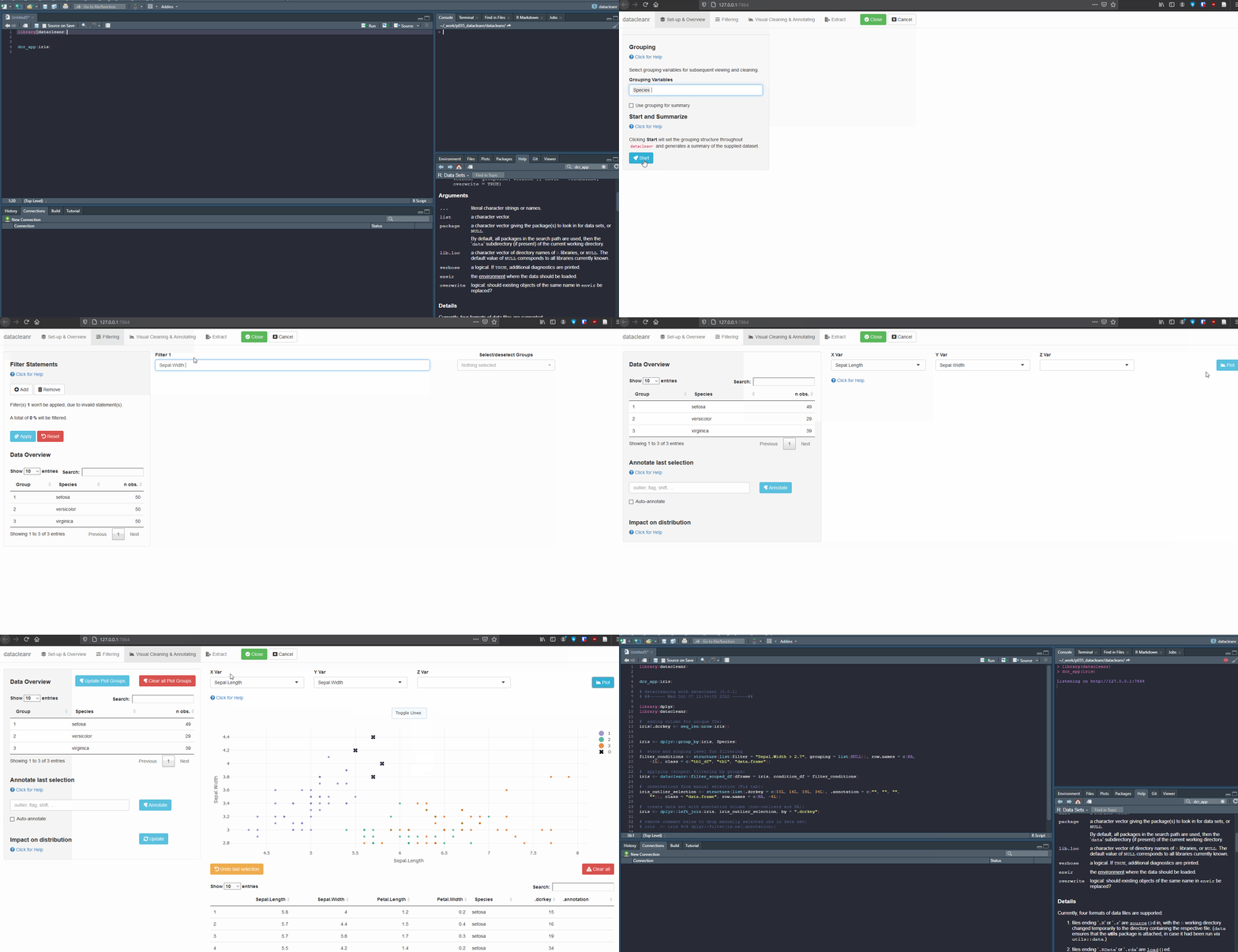
And output from extract tab:
# datacleaning with datacleanr (0.0.1)
# ##------ Wed Oct 07 12:54:03 2020 ------##

library(dplyr)
library(datacleanr)

#  adding column for unique IDs;
iris$.dcrkey <- seq_len(nrow(iris))


iris <- dplyr::group_by(iris, Species)

#  stats and scoping level for filtering
filter_conditions <- structure(list(filter = "Sepal.Width > 2.7", grouping = list(NULL)), row.names = c(NA,
    -1L), class = c("tbl_df", "tbl", "data.frame"))

#  applying (scoped) filtering by groups;
iris <- datacleanr::filter_scoped_df(dframe = iris, condition_df = filter_conditions)

#  observations from manual selection (Viz tab);
iris_outlier_selection <- structure(list(.dcrkey = c(15L, 16L, 19L, 34L), .annotation = c("", "", "",
    "")), class = "data.frame", row.names = c(NA, -4L))

#  create data set with annotation column (non-outliers are NA);
iris <- dplyr::left_join(iris, iris_outlier_selection, by = ".dcrkey")

# remove comment below to drop manually selected obs in data set;
# iris  <- iris %>% dplyr::filter(is.na(.annotation))
Example 2
Launching with an .RDS from disk:
saveRDS(iris, file = "./testiris.Rds")

library(datacleanr)
dcr_app("./testiris.Rds")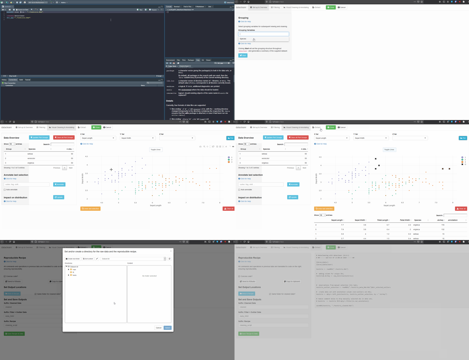
COSORE is a community-driven soil respiration database, recently introduced with a manuscript published here by Bond-Lamberty et al.. The database provides soil respiration flux estimates, as well as meta data across multiple data sets. Let’s explore!
remotes::install_github("bpbond/cosore")
library(dplyr)

# check data base info
db_info <- cosore::csr_database()
tibble::glimpse(db_info)

# grab one data set and explore in detail
dset <- "d20190409_ANJILELI"
anjilleli <- cosore::csr_dataset(dset)
tibble::glimpse(anjilleli$description)


datacleanr::dcr_app(anjilleli$data)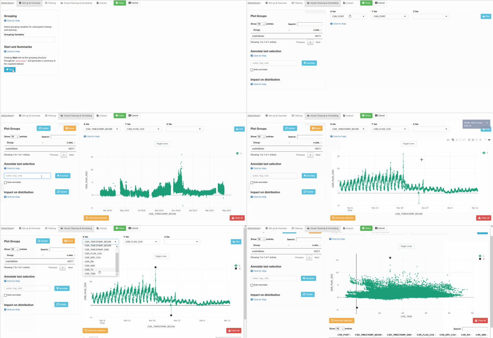
Explore sampling locations:
# Check location info
db_info <- db_info %>%
    mutate(lon = CSR_LONGITUDE,
           lat = CSR_LATITUDE)
datacleanr::dcr_app(db_info)
No GIF
Explore nested data sets:
# grab all data from ZHANG
zhang <- cosore::csr_table("data", c("d20190424_ZHANG_maple",
                                        "d20190424_ZHANG_oak")) %>%
  # adjust for grouping
  mutate(CSR_PORT = as.factor(CSR_PORT))

# group by CSR_DATASET and CSR_PORT
datacleanr::dcr_app(zhang)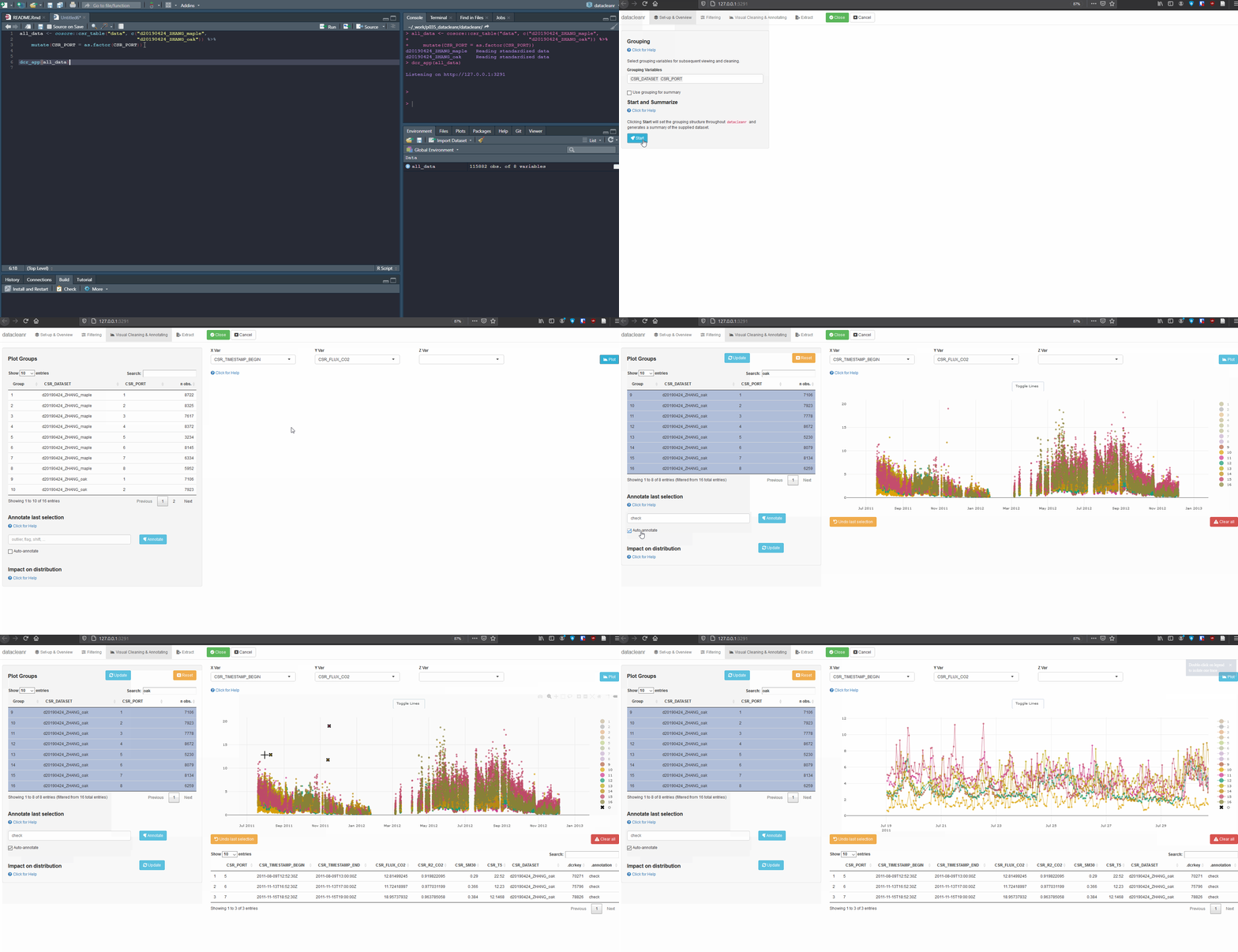
Please note that the datacleanr project is released with
a Contributor
Code of Conduct. By contributing to this project, you agree to abide
by its terms.