discretefit

The package discretefit implements fast Monte Carlo simulations for goodness-of-fit (GOF) tests for discrete distributions. This includes tests based on the root-mean-square statistic, the Chi-squared statistic, the log-likelihood-ratio (G²) statistic, the Freeman-Tukey (Hellinger-distance) statistic, the Kolmogorov-Smirnov statistic, and the Cramer-von Mises statistic.

Simulations are written in C++ (utilizing Rcpp) and are considerably faster than the simulated Chi-squared GOF test in the R stats package.

Installation

You can install discretefit from CRAN.

install.packages("discretefit")

You can also install the development version from GitHub:

devtools::install_github("josh-mc/discretefit")

Usage

The GOF tests in discretefit function on a vector of counts, x, and a vector of probabilities, p. In the below example, x represents a vector of counts for five categories, and p represents a vector of probabilities for each corresponding category. The GOF tests provides p-values for the null hypothesis that x is a random sample of the discrete distribution defined by p. 

library(discretefit)
library(bench)

x <- c(42, 0, 13, 2, 109)
p <- c(0.2, 0.05, 0.1, 0.05, 0.6)

chisq_gof(x, p)
#> 
#>  Simulated Chi-squared goodness-of-fit test
#> 
#> data:  x
#> Chi-squared = 17.082, p-value = 0.0022
rms_gof(x, p)
#> 
#>  Simulated root-mean-square goodness-of-fit test
#> 
#> data:  x
#> RMS = 1.731, p-value = 0.0389
g_gof(x, p)
#> 
#>  Simulated log-likelihood-ratio goodness-of-fit test
#> 
#> data:  x
#> G2 = 27.362, p-value = 9.999e-05
ft_gof(x, p)
#> 
#>  Simulated Freeman-Tukey goodness-of-fit test
#> 
#> data:  x
#> FT = 45.599, p-value = 9.999e-05
ks_gof(x, p)
#> 
#>  Simulated Kolmogorov-Smirnov goodness-of-fit test
#> 
#> data:  x
#> KS = 0.056627, p-value = 0.2404
cvm_gof(x, p)
#> 
#>  Simulated Cramer-von Mises goodness-of-fit test
#> 
#> data:  x
#> W2 = 0.12578, p-value = 0.1784

Speed

The simulated Chi-squared GOF test in discretefit produces identical p-values to the simulated Chi-squared GOF test in the stats package that is part of base R.

set.seed(499)
chisq_gof(x, p, reps = 2000)$p.value
#> [1] 0.002998501
set.seed(499)
chisq.test(x, p = p, simulate.p.value = TRUE)$p.value
#> [1] 0.002998501

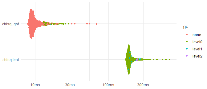
However, because Monte Carlo simulations in discretefit are implemented in C++, chisq_gof is much faster than chisq.test, ~20 times faster for the following case.

speed <- bench::mark(min_iterations = 1000, check = FALSE, 
  chisq_gof = chisq_gof(x, p, reps = 2000),
  chisq.test = chisq.test(x, p = p, simulate.p.value = TRUE, B = 2000)
)
#> Warning: Some expressions had a GC in every iteration; so filtering is disabled.

ggplot2::autoplot(speed) +
  ggplot2::theme_minimal() +
  ggplot2::xlab(NULL) +
  ggplot2::ylab(NULL) 
#> Loading required namespace: tidyr

Additionally, the simulated GOF tests in base R is vectorized, so for large vectors attempting a large number of simulations may not be possible because of memory constraints. Since the functions in discretefit are not vectorized, memory use is minimized.

Root-mean-square statistic

In a surprising number of cases, a simulated GOF test based on the root-mean-square statistic outperforms the Chi-squared test and other tests in the Cressie-Read power divergence family. This has been demonstrated by Perkins, Tygert, and Ward (2011). They provide the following toy example.

Take a discrete distribution with 50 bins (or categories). The probability for the first and second bin is 0.25. The probability for each of the remaining 48 bins is 0.5 / 48 (~0.0104).

Now take the observed counts of 15 for the first bin, 5 for the second bin, and zero for each of the remaining 48 bins. It’s obvious that these observations are very unlikely to occur for a random sample from the above distribution. However, the Chi-squared, G², and Freeman-Tukey tests fail to reject the null hypothesis.

x <- c(15, 5, rep(0, 48))
p <- c(0.25, 0.25, rep(1/(2 * 50 -4), 48))

chisq_gof(x, p)
#> 
#>  Simulated Chi-squared goodness-of-fit test
#> 
#> data:  x
#> Chi-squared = 30, p-value = 0.9681
g_gof(x, p)
#> 
#>  Simulated log-likelihood-ratio goodness-of-fit test
#> 
#> data:  x
#> G2 = 32.958, p-value = 0.6627
ft_gof(x, p)
#> 
#>  Simulated Freeman-Tukey goodness-of-fit test
#> 
#> data:  x
#> FT = 50.718, p-value = 0.141

By contrast, the root-mean-square test convincingly rejects the null hypothesis.

rms_gof(x, p)
#> 
#>  Simulated root-mean-square goodness-of-fit test
#> 
#> data:  x
#> RMS = 5.1042, p-value = 9.999e-05

For additional examples, see Perkins, Tygert, and Ward (2011) and Ward and Carroll (2014).

Alternatives

Several other packages implement GOF tests for discrete distributions.

As noted above, the stats package in base R implements a simulated Chi-squared GOF test.

I’m not aware of an R package that implements a simulated G² GOF test but the packages RVAideMemoire and DescTools implement GOF tests that utilize approximations based on the Chi-squared distribution.

The dgof package (Anderson and Emerson 2011) implements simulated Kolmogorov-Smirnov GOF tests and simulated Cramer-von Mises GOF tests . The cvmdisc package also implements a simulated Cramer-von Mises GOF test.

The KSgeneral package (Dimitrova, Kaishev, and Tan, 2020) implements exact Kolmogorov-Smirnov GOF tests and fast, simulated GOF tests utilizing the algorithm introduced by Wood and Altavela (1978).

I’m not aware of another R package that implements a root-mean-square GOF test.

References

Arnold, Taylor B. and John W. Emerson. “Nonparametric goodness-of-fit tests for discrete null distributions.” R Journal. https://doi.org/10.32614/rj-2011-016

Dimitrova, Dimitrina S., Vladimir K. Kaishev, and Senren Tan. “Computing the Kolmogorov-Smirnov distribution when the underlying CDF is purely discrete, mixed, or continuous.” Journal of Statistical Software, 2020. https://doi.org/10.18637/jss.v095.i10

Eddelbuettel, Dirk and Romain Francois. “Rcpp: Seamless R and C++ Integration.” Journal of Statistical Software, 2011. https://www.jstatsoft.org/article/view/v040i08

Perkins, William, Mark Tygert, and Rachel Ward. “Computing the confidence levels for a root-mean-square test of goodness-of-fit.” Applied Mathematics and Computation, 2011. https://doi.org/10.1016/j.amc.2011.03.124

Ward, Rachel and Raymond J. Carroll. “Testing Hardy–Weinberg equilibrium with a simple root-mean-square statistic.” Biostatistics, 2014. https://doi.org/10.1093/biostatistics/kxt028

Wood, Constance L., and Michele M. Altavela. “Large-Sample Results for Kolmogorov–Smirnov Statistics for Discrete Distributions.” Biometrika, 1978. https://doi.org/10.1093/biomet/65.1.235