ggmeta

ggmeta builds publication-quality forest and funnel plots with ggplot2. Give it a meta object (from the meta package) or a plain tidy data frame — the result is an ordinary ggplot you can theme, compose, and save.

Installation

# install.packages("remotes")
remotes::install_github("drhrf/ggmeta")

Quick start

No meta package required — a tidy data frame of effect sizes and standard errors is enough. Set add_summary = TRUE to pool the studies on the fly (inverse-variance common effect and DerSimonian–Laird random effects):

library(ggmeta)

studies <- data.frame(
  studlab  = c("Trial 1", "Trial 2", "Trial 3", "Trial 4", "Trial 5"),
  estimate = c(0.10, 0.35, 0.22, 0.48, 0.05),
  se       = c(0.12, 0.10, 0.14, 0.16, 0.11)
)
studies$ci_lower <- studies$estimate - 1.96 * studies$se
studies$ci_upper <- studies$estimate + 1.96 * studies$se

ggforest(studies, add_summary = TRUE)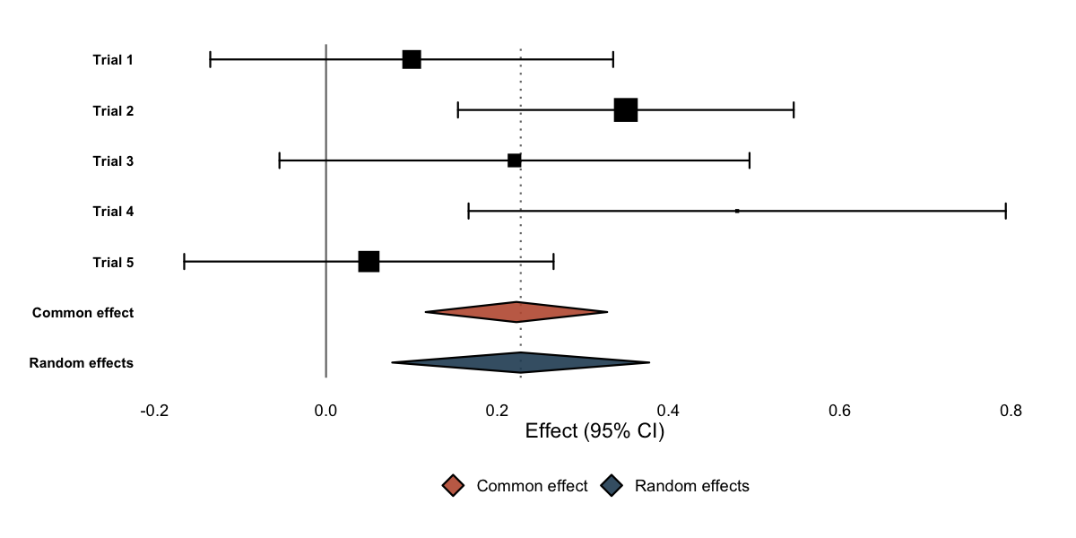

Estimates, CIs, weights, and heterogeneity

Pass a meta object and add columns = TRUE to reproduce the familiar meta::forest() table: an effect estimate, 95% CI, and weight column for every study and summary, headers, and a heterogeneity line (I², the between-study variance, Q, and p) — all as a plain ggplot.

library(meta)
#> Loading required package: metabook
#> Loading 'meta' package (version 8.5-0).
#> Type 'help(meta)' for a brief overview.

dat <- data.frame(
  study   = c("Adams 2019", "Baker 2020", "Chen 2020",
              "Diaz 2021", "Evans 2022", "Foster 2023"),
  event.e = c(12,  8, 25, 18, 30, 15), n.e = c(120,  90, 200, 150, 250, 130),
  event.c = c(20, 14, 30, 28, 35, 25), n.c = c(118,  92, 205, 148, 245, 128)
)

m <- metabin(event.e, n.e, event.c, n.c,
             data = dat, studlab = study, sm = "RR")

ggforest(m, columns = TRUE)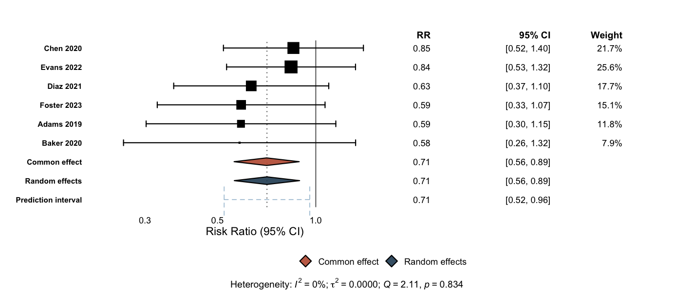

Everything is optional. Choose which columns to show, and toggle the other elements on or off:

ggforest(m, columns = c("estimate", "ci")) # only some columns
ggforest(m, effect_header = "Risk ratio")  # rename the estimate column
ggforest(m, show_hetstats = FALSE)          # hide the heterogeneity line
ggforest(m, show_predict  = FALSE)          # hide the prediction interval
ggforest(m, sort_studies  = FALSE)          # keep the input order

Forest and funnel plots on one canvas

ggmeta also draws funnel plots with ggfunnel() (study effect vs. standard error, with pseudo confidence-interval contours). And because every plot is an ordinary ggplot, a forest and a funnel compose on a single figure with patchwork — something that is awkward with the base-graphics output of meta:

library(patchwork)

(ggforest(m) | ggfunnel(m)) +
  plot_layout(widths = c(2, 1)) +
  plot_annotation(tag_levels = "A")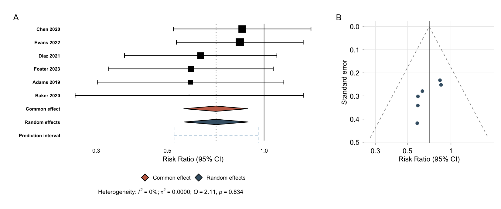

Journal styles

Layout presets restyle a plot for common journals. They are ordinary ggplot2 components, so you add them with +:

layout_jama(ggforest(m, columns = TRUE))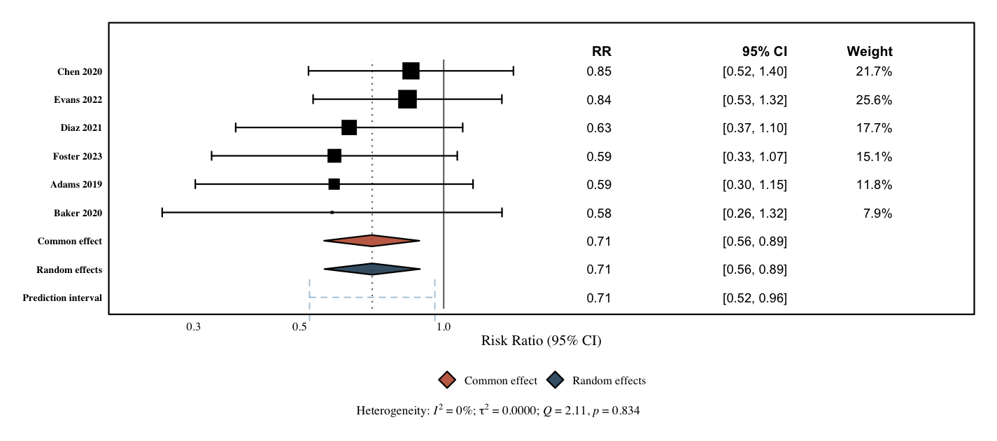

layout_bmj() and layout_revman5() are also available.

Custom columns

For a column of your own — sample sizes, events, anything — use geom_forest_text(), aligned to the study rows through the shared y. tidy_meta() exposes the same tidy data frame ggforest() builds internally, and format_effect() builds "estimate (low to high)" labels:

td      <- tidy_meta(m)
studies <- td[!td$is_summary, ]

ggforest(m) +
  geom_forest_text(aes(y = studlab, label = n.e), data = studies,
                   x = 4, hjust = 0) +
  expand_limits(x = 6)

Why ggmeta?

• ggplot2 native — add themes, layers, annotations, and facets; save with ggsave().
• Forest and funnel plots — ggforest() and ggfunnel(), both ordinary ggplots, so you can arrange them together with patchwork.
• meta::forest()-style tables — estimate / CI / weight columns and a heterogeneity caption, via columns = TRUE.
• Standalone or meta — works on a tidy data frame or a meta object, and can pool studies itself (add_summary = TRUE).
• Correct by construction — every summary measure is back-transformed with its right inverse (ratios, logit proportions, Fisher-z correlations, rates).
• Custom geometries — proper ggproto geoms for CIs, summary diamonds, prediction intervals, reference lines, and text columns.
• Journal styles — layout_jama(), layout_bmj(), layout_revman5().

Learn more

• vignette("getting-started") — a tour of the package.
• vignette("customising") — restyle every element of a forest or funnel plot.
• vignette("from-meta-forest") — coming from meta::forest().