
giscoR is an R package that provides a simple interface to GISCO data from Eurostat. It allows you to download and work with global and European geospatial datasets (such as country boundaries, NUTS regions, coastlines, and labels) directly in R.
60M,
20M, 10M, 03M,
01M.Install giscoR from CRAN:
install.packages("giscoR")Check the docs of the developing version in https://ropengov.github.io/giscoR/dev/.
You can install the development version of giscoR with:
# install.packages("pak")

pak::pak("rOpenGov/giscoR")
Alternatively, you can install giscoR via r-universe:
install.packages(
  "giscoR",
  repos = c("https://ropengov.r-universe.dev", "https://cloud.r-project.org")
)This script highlights some features of giscoR:
library(giscoR)
library(sf)
library(dplyr)

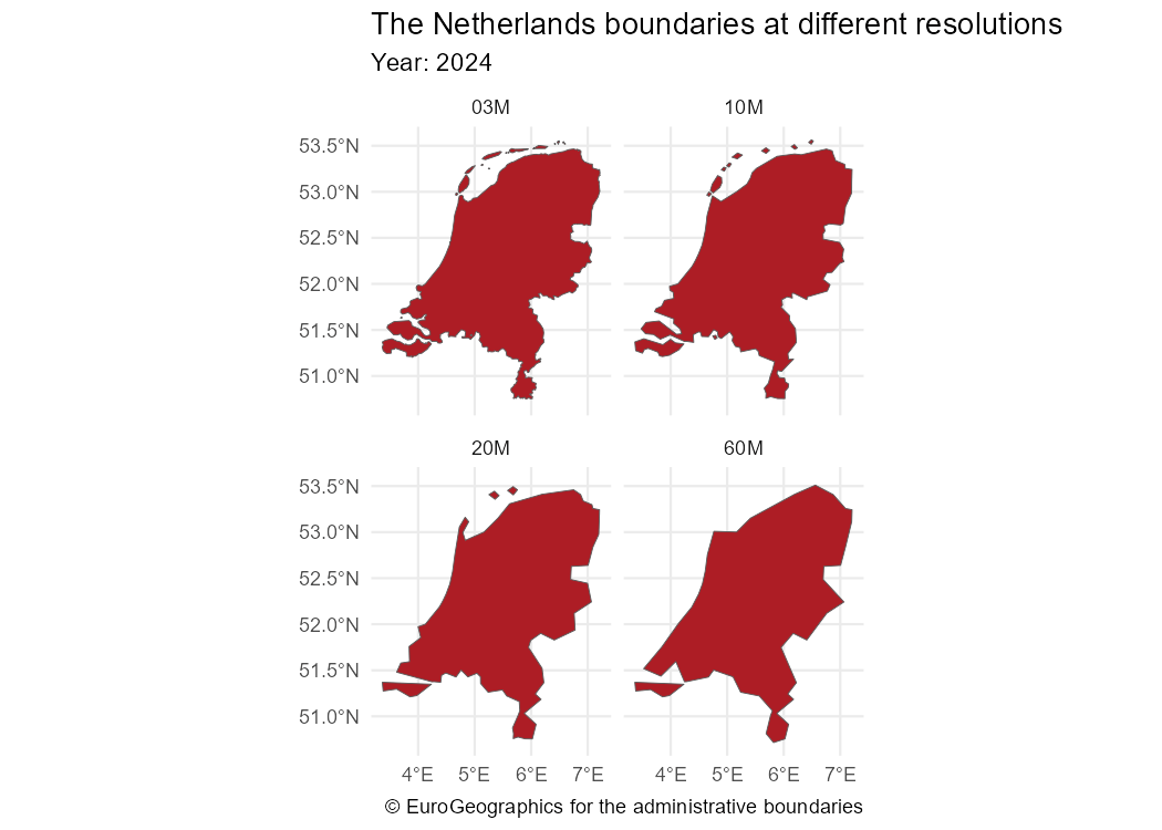
# Download The Netherlands boundaries at different resolutions
nl_all <- lapply(c("60", "20", "10", "03"), function(r) {
  gisco_get_countries(country = "Netherlands", year = 2024, resolution = r) |>
    mutate(res = paste0(r, "M"))
}) |>
  bind_rows()

glimpse(nl_all)
#> Rows: 4
#> Columns: 13
#> $ CNTR_ID   <chr> "NL", "NL", "NL", "NL"
#> $ CNTR_NAME <chr> "Nederland", "Nederland", "Nederland", "Nederland"
#> $ NAME_ENGL <chr> "Netherlands", "Netherlands", "Netherlands", "Netherlands"
#> $ NAME_FREN <chr> "Pays-Bas", "Pays-Bas", "Pays-Bas", "Pays-Bas"
#> $ ISO3_CODE <chr> "NLD", "NLD", "NLD", "NLD"
#> $ SVRG_UN   <chr> "UN Member State", "UN Member State", "UN Member State", "UN…
#> $ CAPT      <chr> "Amsterdam", "Amsterdam", "Amsterdam", "Amsterdam"
#> $ EU_STAT   <chr> "T", "T", "T", "T"
#> $ EFTA_STAT <chr> "F", "F", "F", "F"
#> $ CC_STAT   <chr> "F", "F", "F", "F"
#> $ NAME_GERM <chr> "Niederlande", "Niederlande", "Niederlande", "Niederlande"
#> $ res       <chr> "60M", "20M", "10M", "03M"
#> $ geometry  <MULTIPOLYGON [°]> MULTIPOLYGON (((7.208935 53..., MULTIPOLYGON (((7.202794 53.…

# Plot with ggplot2

library(ggplot2)

ggplot(nl_all) +
  geom_sf(fill = "#AD1D25") +
  facet_wrap(~res) +
  labs(
    title = "The Netherlands boundaries at different resolutions",
    subtitle = "Year: 2024",
    caption = gisco_attributions()
  ) +
  theme_minimal()
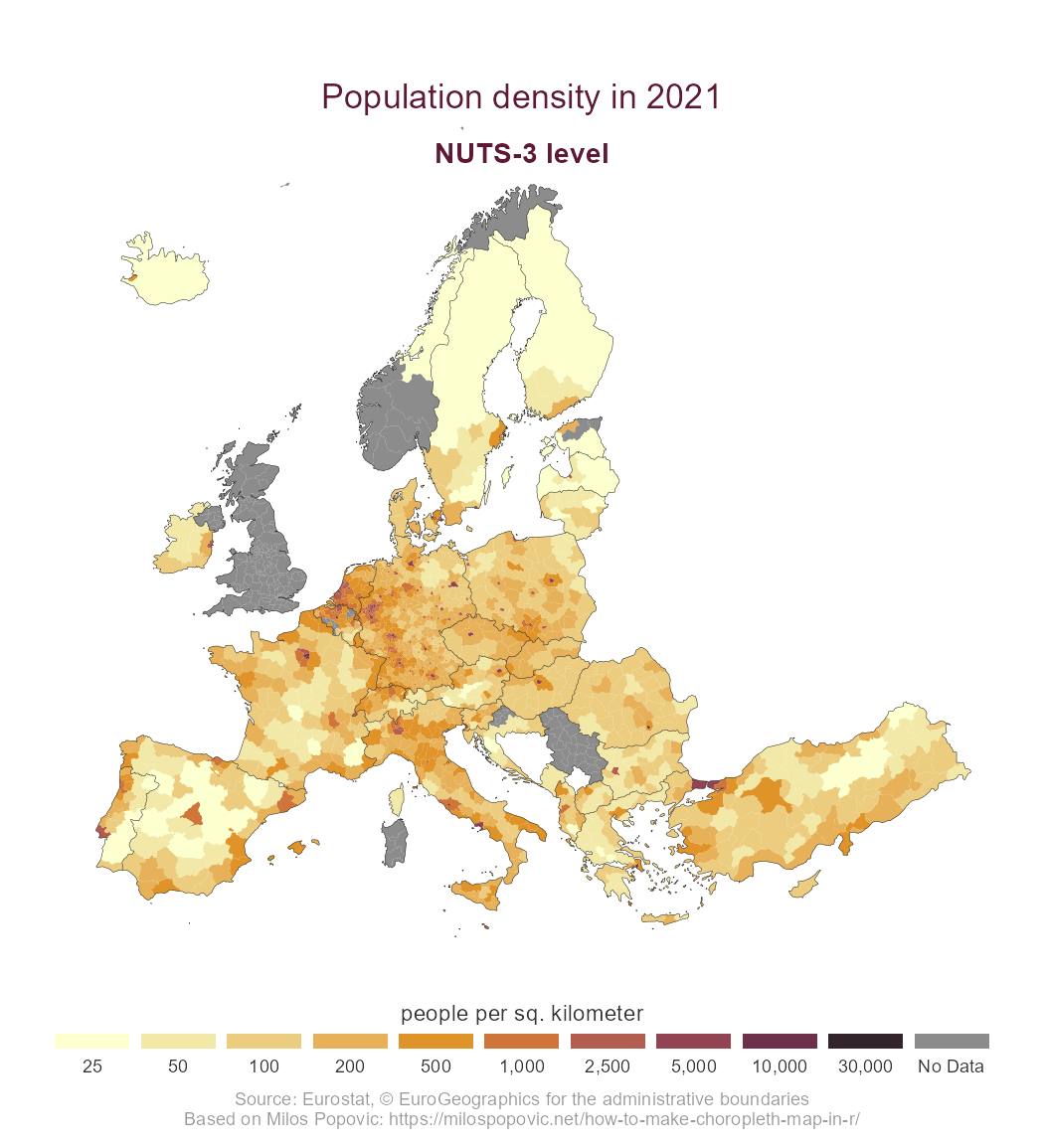
This example shows a thematic map created with the ggplot2 package. The data are obtained via the eurostat package. This follows the work of Milos Popovic.
We start by extracting the corresponding geographic data:
library(giscoR)
library(dplyr)
library(eurostat)
library(ggplot2)

# Get sf objects
nuts3 <- gisco_get_nuts(
  year = 2021,
  epsg = 3035,
  resolution = 10,
  nuts_level = 3
)

# Get country lines (NUTS 0 level)

country_lines <- gisco_get_nuts(
  year = 2021,
  epsg = 3035,
  resolution = 10,
  spatialtype = "BN",
  nuts_level = 0
)
We now download the data from Eurostat:
# Use eurostat
popdens <- get_eurostat("demo_r_d3dens") |>
  filter(TIME_PERIOD == "2021-01-01")
#>
indexed 0B in  0s, 0B/s
indexed 2.15GB in  0s, 2.15GB/s
Finally, we merge and manipulate the data to create the final plot:
# Merge data
nuts3_sf <- nuts3 |>
  left_join(popdens, by = "geo")

# Breaks and labels
br <- c(0, 25, 50, 100, 200, 500, 1000, 2500, 5000, 10000, 30000)
labs <- prettyNum(br[-1], big.mark = ",")

# Label function used in the plot, mainly for NAs
labeller_plot <- function(x) {
  ifelse(is.na(x), "No Data", x)
}
nuts3_sf <- nuts3_sf |>
  # Cut with labels
  mutate(values_cut = cut(values, br, labels = labs))


# Palette
pal <- hcl.colors(length(labs), "Lajolla")


# Plot
ggplot(nuts3_sf) +
  geom_sf(aes(fill = values_cut), linewidth = 0, color = NA, alpha = 0.9) +
  geom_sf(data = country_lines, col = "black", linewidth = 0.1) +
  # Center in Europe: EPSG 3035
  coord_sf(
    xlim = c(2377294, 7453440),
    ylim = c(1313597, 5628510)
  ) +
  # Legends
  scale_fill_manual(
    values = pal,
    # Label for NA
    labels = labeller_plot,
    drop = FALSE,
    guide = guide_legend(direction = "horizontal", nrow = 1)
  ) +
  # Theming
  theme_void() +
  # Theme
  theme(
    plot.title = element_text(
      color = rev(pal)[2],
      size = rel(1.5),
      hjust = 0.5,
      vjust = -6
    ),
    plot.subtitle = element_text(
      color = rev(pal)[2],
      size = rel(1.25),
      hjust = 0.5,
      vjust = -10,
      face = "bold"
    ),
    plot.caption = element_text(color = "grey60", hjust = 0.5, vjust = 0),
    legend.text = element_text(color = "grey20", hjust = 0.5),
    legend.title = element_text(color = "grey20", hjust = 0.5),
    legend.position = "bottom",
    legend.title.position = "top",
    legend.text.position = "bottom",
    legend.key.height = unit(0.5, "line"),
    legend.key.width = unit(2.5, "line")
  ) +
  # Annotate and labs
  labs(
    title = "Population density in 2021",
    subtitle = "NUTS-3 level",
    fill = "people per sq. kilometer",
    caption = paste0(
      "Source: Eurostat, ",
      gisco_attributions(),
      "\nBased on Milos Popovic's work"
    )
  )
Large datasets (e.g., LAU or high-resolution files) can exceed 50MB. Use:
gisco_set_cache_dir("./path/to/location")Files will be stored locally for faster access.
Check the GitHub page for source code.
Contributions are welcome:
To cite ‘giscoR’ in publications use:
Hernangómez D (2026). giscoR: Download Map Data from GISCO API - Eurostat. doi:10.32614/CRAN.package.giscoR https://doi.org/10.32614/CRAN.package.giscoR, https://ropengov.github.io/giscoR/.
A BibTeX entry for LaTeX users is
@Manual{R-giscoR,
  title = {{giscoR}: Download Map Data from GISCO API - Eurostat},
  doi = {10.32614/CRAN.package.giscoR},
  author = {Diego Hernangómez},
  year = {2026},
  version = {1.1.0},
  url = {https://ropengov.github.io/giscoR/},
  abstract = {Tools to download data from the GISCO (Geographic Information System of the Commission) Eurostat database <https://ec.europa.eu/eurostat/web/gisco>. Global and European map data available. This package is in no way officially related to or endorsed by Eurostat.},
}Eurostat’s general copyright notice and licence policy applies. Moreover, there are specific rules that apply to some of the following datasets available for downloading. The download and use of these data are subject to these rules being accepted. See our administrative units and statistical units for more details.
This package is neither affiliated with nor endorsed by Eurostat. The authors are not responsible for any misuse of the data.