A package for getting the most out of large multilevel models in R
by Jared E. Knowles and Carl Frederick
Working with generalized linear mixed models (GLMM) and linear mixed
models (LMM) has become increasingly easy with advances in the
lme4 package. As we have found ourselves using these models
more and more within our work, we, the authors, have developed a set of
tools for simplifying and speeding up common tasks for interacting with
merMod objects from lme4. This package
provides those tools.
# development version
library(devtools)
install_github("jknowles/merTools")

# CRAN version
install.packages("merTools")merTools as feature
complete. The package now enters maintenance
mode: future releases will focus on bug fixes, dependency and
CRAN compatibility, and documentation rather than new features.predictInterval() on nested random effects (#124), a
repaired and extended shinyMer() (#32, #78), the new
plotREimpact() plot (#84, #85), and refreshed documentation
(#116, #136, #137). See NEWS.md for the full list.vctrs package impacting
dplyr::bind_rows() usage in REsim (#133)vcov in the
merDeriv packageaes_string() calls (#127)subBoot now works with glmerMod objects as
wellreMargins a new function that allows the user to
marginalize the prediction over breaks in the distribution of random
effect distributions, see ?reMargins and the new
reMargins vignette (closes #73)merModList functions now
apply the Rubin correction for multiple imputationThe easiest way to demo the features of this application is to use the bundled Shiny application which launches a number of the metrics here to aide in exploring the model. To do this:
library(merTools)
m1 <- lmer(y ~ service + lectage + studage + (1|d) + (1|s), data=InstEval)
shinyMer(m1, simData = InstEval[1:100, ]) # just try the first 100 rows of data
On the first tab, the function presents the prediction intervals for
the data selected by user which are calculated using the
predictInterval function within the package. This function
calculates prediction intervals quickly by sampling from the simulated
distribution of the fixed effect and random effect terms and combining
these simulated estimates to produce a distribution of predictions for
each observation. This allows prediction intervals to be generated from
very large models where the use of bootMer would not be
feasible computationally.

On the next tab the distribution of the fixed effect and group-level
effects is depicted on confidence interval plots. These are useful for
diagnostics and provide a way to inspect the relative magnitudes of
various parameters. This tab makes use of four related functions in
merTools: FEsim, plotFEsim,
REsim and plotREsim which are available to be
used on their own as well.

On the third tab are some convenient ways to show the influence or
magnitude of effects by leveraging the power of
predictInterval. For each case, up to 12, in the selected
data type, the user can view the impact of changing either one of the
fixed effect or one of the grouping level terms. Using the
REimpact function, each case is simulated with the model’s
prediction if all else was held equal, but the observation was moved
through the distribution of the fixed effect or the random effect term.
This is plotted on the scale of the dependent variable, which allows the
user to compare the magnitude of effects across variables, and also
between models on the same data.
Standard prediction looks like so.
predict(m1, newdata = InstEval[1:10, ])
#>        1        2        3        4        5        6        7        8
#> 3.146337 3.165212 3.398499 3.114249 3.320686 3.252670 4.180897 3.845219
#>        9       10
#> 3.779337 3.331013
With predictInterval we obtain predictions that are more
like the standard objects produced by lm and
glm:
predictInterval(m1, newdata = InstEval[1:10, ], n.sims = 500, level = 0.9,
                stat = 'median')
#>         fit      upr      lwr
#> 1  3.161371 5.103826 1.139883
#> 2  3.232387 5.009761 1.332832
#> 3  3.445031 5.291794 1.499974
#> 4  3.013080 5.244352 1.104054
#> 5  3.291172 5.228658 1.150961
#> 6  3.311819 5.336952 1.060889
#> 7  4.165035 5.971790 2.084237
#> 8  3.830382 5.578582 1.791503
#> 9  3.801973 5.845741 1.924566
#> 10 3.358777 5.288322 1.581321
Note that predictInterval is slower because it is
computing simulations. It can also return all of the simulated
yhat values as an attribute to the predict object
itself.
predictInterval uses the sim function from
the arm package heavily to draw the distributions of the
parameters of the model. It then combines these simulated values to
create a distribution of the yhat for each observation.
We can also explore the components of the prediction interval by
asking predictInterval to return specific components of the
prediction interval.
predictInterval(m1, newdata = InstEval[1:10, ], n.sims = 200, level = 0.9,
                stat = 'median', which = "all")
#>      effect          fit      upr        lwr obs
#> 1  combined  3.083593245 5.062599  0.9674464   1
#> 2  combined  3.235036697 5.212885  1.1708064   2
#> 3  combined  3.342847853 5.371818  1.2686879   3
#> 4  combined  3.077033326 5.251489  1.3107275   4
#> 5  combined  3.316029839 5.337122  1.4697923   5
#> 6  combined  3.443738022 5.172142  0.9068009   6
#> 7  combined  4.112843798 6.535431  2.1650584   7
#> 8  combined  3.816085776 5.974373  1.8064576   8
#> 9  combined  3.792304602 5.609345  1.8844468   9
#> 10 combined  3.333815423 5.402147  1.5005593  10
#> 11        s  0.231536444 1.790168 -1.7006576   1
#> 12        s  0.134265072 1.957335 -1.7931547   2
#> 13        s  0.218560304 2.021749 -1.7836963   3
#> 14        s -0.099702591 2.029545 -1.8110851   4
#> 15        s -0.045505671 1.693573 -2.1095589   5
#> 16        s -0.087337382 1.716194 -2.0527377   6
#> 17        s  0.376170634 2.109191 -1.8125491   7
#> 18        s  0.364157813 2.329252 -1.4930631   8
#> 19        s  0.415591035 2.240454 -1.4130724   9
#> 20        s  0.356965891 2.283956 -1.7016778  10
#> 21        d  0.008946287 1.700966 -2.0450912   1
#> 22        d -0.095226122 1.741526 -2.0126363   2
#> 23        d -0.171781743 2.068428 -2.2161950   3
#> 24        d -0.225090139 1.962778 -2.2287493   4
#> 25        d  0.242943045 2.185860 -1.5681800   5
#> 26        d -0.083381572 1.958019 -2.1527131   6
#> 27        d  0.505729236 2.272959 -1.0985370   7
#> 28        d  0.223848219 1.892653 -1.4133758   8
#> 29        d  0.232838207 2.161019 -1.6092655   9
#> 30        d -0.411865471 1.744540 -2.4933411  10
#> 31    fixed  3.102540070 5.098888  1.2745417   1
#> 32    fixed  3.071049868 5.045066  1.1160584   2
#> 33    fixed  3.325102518 5.242442  1.1231595   3
#> 34    fixed  3.185105756 4.766187  1.1267020   4
#> 35    fixed  3.392547857 4.902974  1.3989885   5
#> 36    fixed  3.213560141 4.949743  1.2420229   6
#> 37    fixed  3.197190288 5.109854  1.1668196   7
#> 38    fixed  3.305944109 5.132413  1.5010800   8
#> 39    fixed  3.395006368 5.327011  1.7248772   9
#> 40    fixed  3.415382668 5.052743  1.1706732  10
This can lead to some useful plotting:
library(ggplot2)
plotdf <- predictInterval(m1, newdata = InstEval[1:10, ], n.sims = 2000,
                          level = 0.9, stat = 'median', which = "all",
                          include.resid.var = FALSE)
plotdfb <- predictInterval(m1, newdata = InstEval[1:10, ], n.sims = 2000,
                          level = 0.9, stat = 'median', which = "all",
                          include.resid.var = TRUE)

plotdf <- dplyr::bind_rows(plotdf, plotdfb, .id = "residVar")
plotdf$residVar <- ifelse(plotdf$residVar == 1, "No Model Variance",
                          "Model Variance")

ggplot(plotdf, aes(x = obs, y = fit, ymin = lwr, ymax = upr)) +
  geom_pointrange() +
  geom_hline(yintercept = 0, color = I("red"), size = 1.1) +
  scale_x_continuous(breaks = c(1, 10)) +
  facet_grid(residVar~effect) + theme_bw()
#> Warning: Using `size` aesthetic for lines was deprecated in ggplot2 3.4.0.
#> ℹ Please use `linewidth` instead.
#> This warning is displayed once per session.
#> Call `lifecycle::last_lifecycle_warnings()` to see where this warning was
#> generated.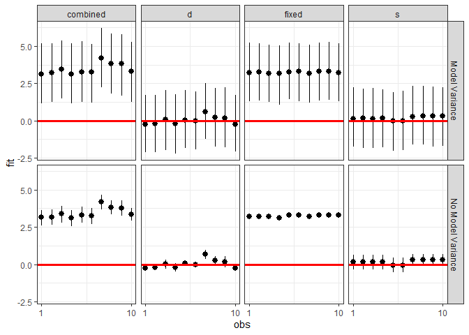
We can also investigate the makeup of the prediction for each observation.
ggplot(plotdf[plotdf$obs < 6,],
       aes(x = effect, y = fit, ymin = lwr, ymax = upr)) +
  geom_pointrange() +
  geom_hline(yintercept = 0, color = I("red"), size = 1.1) +
  facet_grid(residVar~obs) + theme_bw()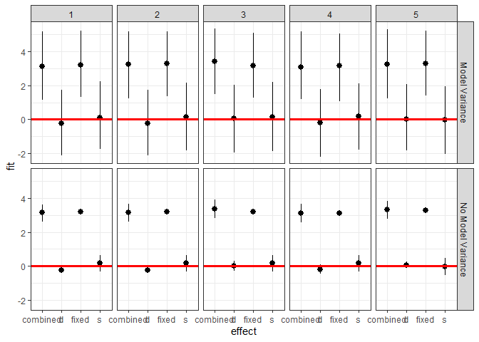
merTools also provides functionality for inspecting
merMod objects visually. The easiest are getting the
posterior distributions of both fixed and random effect parameters.
feSims <- FEsim(m1, n.sims = 100)
head(feSims)
#>          term        mean      median         sd
#> 1 (Intercept)  3.22480254  3.22496233 0.01614456
#> 2    service1 -0.06978571 -0.07023666 0.01257453
#> 3   lectage.L -0.18553409 -0.18582412 0.01558176
#> 4   lectage.Q  0.02485585  0.02585718 0.01197095
#> 5   lectage.C -0.02587443 -0.02424027 0.01327372
#> 6   lectage^4 -0.02253842 -0.02115560 0.01434107
And we can also plot this:
plotFEsim(FEsim(m1, n.sims = 100), level = 0.9, stat = 'median', intercept = FALSE)
We can also quickly make caterpillar plots for the random-effect terms:
reSims <- REsim(m1, n.sims = 100)
head(reSims)
#>   groupFctr groupID        term         mean      median        sd
#> 1         s       1 (Intercept)  0.148244481 0.170819888 0.3386784
#> 2         s       2 (Intercept) -0.006549032 0.009520074 0.3202212
#> 3         s       3 (Intercept)  0.264735849 0.268038770 0.2765385
#> 4         s       4 (Intercept)  0.259182685 0.242682150 0.3018633
#> 5         s       5 (Intercept)  0.020047123 0.019007888 0.3068737
#> 6 s 6 (Intercept) 0.081449654 0.078937547 0.2519452plotREsim(REsim(m1, n.sims = 100), stat = 'median', sd = TRUE)
Note that plotREsim highlights group levels that have a
simulated distribution that does not overlap 0 – these appear darker.
The lighter bars represent grouping levels that are not distinguishable
from 0 in the data.
Sometimes the random effects can be hard to interpret and not all of
them are meaningfully different from zero. To help with this
merTools provides the expectedRank function,
which provides the percentile ranks for the observed groups in the
random effect distribution taking into account both the magnitude and
uncertainty of the estimated effect for each group.
ranks <- expectedRank(m1, groupFctr = "d")
head(ranks)
#>   groupFctr groupLevel      term   estimate  std.error       ER pctER
#> 2         d          1 Intercept  0.3944919 0.08665152 835.3005    74
#> 3         d          6 Intercept -0.4428949 0.03901988 239.5363    21
#> 4         d          7 Intercept  0.6562681 0.03717200 997.3569    88
#> 5         d          8 Intercept -0.6430680 0.02210017 138.3445    12
#> 6         d         12 Intercept  0.1902940 0.04024063 702.3410    62
#> 7         d         13 Intercept  0.2497464 0.03216255 750.0174    66
A nice features expectedRank is that you can return the
expected rank for all factors simultaneously and use them:
ranks <- expectedRank(m1)
head(ranks)
#>   groupFctr groupLevel      term    estimate  std.error       ER pctER
#> 2         s          1 Intercept  0.16732800 0.08165665 1931.570    65
#> 3         s          2 Intercept -0.04409538 0.09234250 1368.160    46
#> 4         s          3 Intercept  0.30382219 0.05204082 2309.941    78
#> 5         s          4 Intercept  0.24756175 0.06641699 2151.828    72
#> 6         s          5 Intercept  0.05232329 0.08174130 1627.693    55
#> 7         s          6 Intercept  0.10191653 0.06648394 1772.548    60

ggplot(ranks, aes(x = term, y = estimate)) +
  geom_violin(fill = "gray50") + facet_wrap(~groupFctr) +
  theme_bw()
It can still be difficult to interpret the results of LMM and GLMM
models, especially the relative influence of varying parameters on the
predicted outcome. This is where the REimpact and the
wiggle functions in merTools can be handy.
impSim <- REimpact(m1, InstEval[7, ], groupFctr = "d", breaks = 5,
                   n.sims = 300, level = 0.9)
#> Warning: executing %dopar% sequentially: no parallel backend registered
impSim
#>   case bin   AvgFit     AvgFitSE nobs
#> 1    1   1 2.780092 3.023753e-04  193
#> 2    1   2 3.253589 6.367631e-05  240
#> 3    1   3 3.545126 5.249834e-05  254
#> 4    1   4 3.829405 6.408711e-05  265
#> 5    1   5 4.232709 1.919177e-04  176
The result of REimpact shows the change in the
yhat as the case we supplied to newdata is
moved from the first to the fifth quintile in terms of the magnitude of
the group factor coefficient. We can see here that the individual
professor effect has a strong impact on the outcome variable. The new
plotREimpact() function visualizes this directly:
plotREimpact(impSim)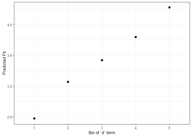
Here the standard error is a bit different – it is the weighted
standard error of the mean effect within the bin. It does not take into
account the variability within the effects of each observation in the
bin – accounting for this variation will be a future addition to
merTools. ### Comparing grouping factors with
plotREimpact()
New in merTools 1.0.0, plotREimpact() plots
REimpact() output directly and can overlay a named
list of results on a single chart. This makes it easy to compare
how strongly different grouping factors move the predicted outcome for
the same case – here, the instructor (d) and student
(s) effects from the model above:
s_impSim <- REimpact(m1, InstEval[7, ], groupFctr = "s", breaks = 5,
                     n.sims = 300, level = 0.9)
plotREimpact(list("Instructor (d)" = impSim, "Student (s)" = s_impSim))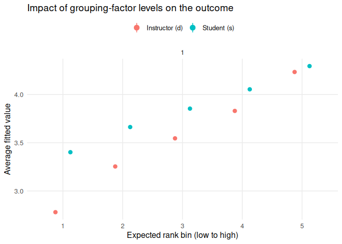
Another feature of merTools is the ability to easily
generate hypothetical scenarios to explore the predicted outcomes of a
merMod object and understand what the model is saying in
terms of the outcome variable.
Let’s take the case where we want to explore the impact of a model with an interaction term between a category and a continuous predictor. First, we fit a model with interactions:
data(VerbAgg)
fmVA <- glmer(r2 ~ (Anger + Gender + btype + situ)^2 +
           (1|id) + (1|item), family = binomial,
           data = VerbAgg)
#> Warning in checkConv(attr(opt, "derivs"), opt$par, ctrl = control$checkConv, : Model failed to converge with max|grad| = 0.0729926 (tol = 0.002, component 1)
#>   See ?lme4::convergence and ?lme4::troubleshooting.
Now we prep the data using the draw function in
merTools. Here we draw the average observation from the
model frame. We then wiggle the data by expanding the
dataframe to include the same observation repeated but with different
values of the variable specified by the var parameter.
Here, we expand the dataset to all values of btype,
situ, and Anger subsequently.
# Select the average case
newData <- draw(fmVA, type = "average")
newData <- wiggle(newData, varlist = "btype",
                  valueslist = list(unique(VerbAgg$btype)))
newData <- wiggle(newData, var = "situ",
                  valueslist = list(unique(VerbAgg$situ)))
newData <- wiggle(newData, var = "Anger",
                  valueslist = list(unique(VerbAgg$Anger)))
head(newData, 10)
#>    r2 Anger Gender btype  situ  id        item
#> 1   N    20      F curse other 149 S3WantCurse
#> 2   N    20      F scold other 149 S3WantCurse
#> 3   N    20      F shout other 149 S3WantCurse
#> 4   N    20      F curse  self 149 S3WantCurse
#> 5   N    20      F scold  self 149 S3WantCurse
#> 6   N    20      F shout  self 149 S3WantCurse
#> 7   N    11      F curse other 149 S3WantCurse
#> 8   N    11      F scold other 149 S3WantCurse
#> 9   N    11      F shout other 149 S3WantCurse
#> 10  N    11      F curse  self 149 S3WantCurse
The next step is familiar – we simply pass this new dataset to
predictInterval in order to generate predictions for these
counterfactuals. Then we plot the predicted values against the
continuous variable, Anger, and facet and group on the two
categorical variables situ and btype
respectively.
plotdf <- predictInterval(fmVA, newdata = newData, type = "probability",
            stat = "median", n.sims = 1000)
#> Warning: For binomial GLMMs, include.resid.var = TRUE simulates from the
#> conditional binomial distribution (n-trial binomial simulation).
#> This is the theoretically correct approach.
#> To get predictions without residual variance, set include.resid.var = FALSE.
plotdf <- cbind(plotdf, newData)

ggplot(plotdf, aes(y = fit, x = Anger, color = btype, group = btype)) +
  geom_point() + geom_smooth(aes(color = btype), method = "lm") +
  facet_wrap(~situ) + theme_bw() +
  labs(y = "Predicted Probability")
#> `geom_smooth()` using formula = 'y ~ x'
predictInterval() is stochastic, so the usual unit-test
tolerances are not a reliable way to confirm that a refactor of the
simulation internals has preserved numeric behavior for users who rely
on a fixed seed. To address this, the package ships a standalone
regression harness that pins a canonical set of inputs (LMM and GLMM
models, various which, level,
stat, ignore.fixed.terms,
fix.intercept.variance, and single-row-newdata cases) and
dumps predictInterval() output to an RDS bundle for two
package versions so they can be diffed bit-for-bit.
The script lives at
tests/comparisons/predictInterval-regression.R and is NOT
part of R CMD check. It has two modes:
# Generate an output bundle for one package version
Rscript tests/comparisons/predictInterval-regression.R harness \
        <pkg_path> <output.rds>

# Diff two bundles
Rscript tests/comparisons/predictInterval-regression.R diff \
        <a.rds> <b.rds>
Typical workflow — comparing the current checkout against
origin/master:
git worktree add /tmp/mT-old origin/master
Rscript tests/comparisons/predictInterval-regression.R harness /tmp/mT-old /tmp/old.rds
Rscript tests/comparisons/predictInterval-regression.R harness .          /tmp/new.rds
Rscript tests/comparisons/predictInterval-regression.R diff  /tmp/old.rds /tmp/new.rds
git worktree remove /tmp/mT-old
The diff output categorizes every case as IDENTICAL,
numeric-equal (< 1e-6), or various drift tiers. Any LMM
case showing more than numeric-equal indicates that the
refactor changed behavior for a user-supplied seed and should be
investigated before the change is merged. Known-intentional numeric
differences (for example, the GLMM include.resid.var = TRUE
binomial-residual simulation fix introduced in 0.9.0) will show up only
in the two glmm_bin_with_resid_* cases.
Run this whenever touching R/merPredict.R,
R/predictInterval_helpers.R, or the simulation helpers they
call.
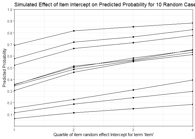
# get cases
case_idx <- sample(1:nrow(VerbAgg), 10)
mfx <- REmargins(fmVA, newdata = VerbAgg[case_idx,], breaks = 4, groupFctr = "item",
                 type = "probability")
#> Warning: For binomial GLMMs, include.resid.var = TRUE simulates from the
#> conditional binomial distribution (n-trial binomial simulation).
#> This is the theoretically correct approach.
#> To get predictions without residual variance, set include.resid.var = FALSE.

ggplot(mfx, aes(y = fit_combined, x = breaks, group = case)) +
  geom_point() + geom_line() +
  theme_bw() +
  scale_y_continuous(breaks = 1:10/10, limits = c(0, 1)) +
  coord_cartesian(expand = FALSE) +
  labs(x = "Quartile of item random effect Intercept for term 'item'",
       y = "Predicted Probability",
       title = "Simulated Effect of Item Intercept on Predicted Probability for 10 Random Cases")