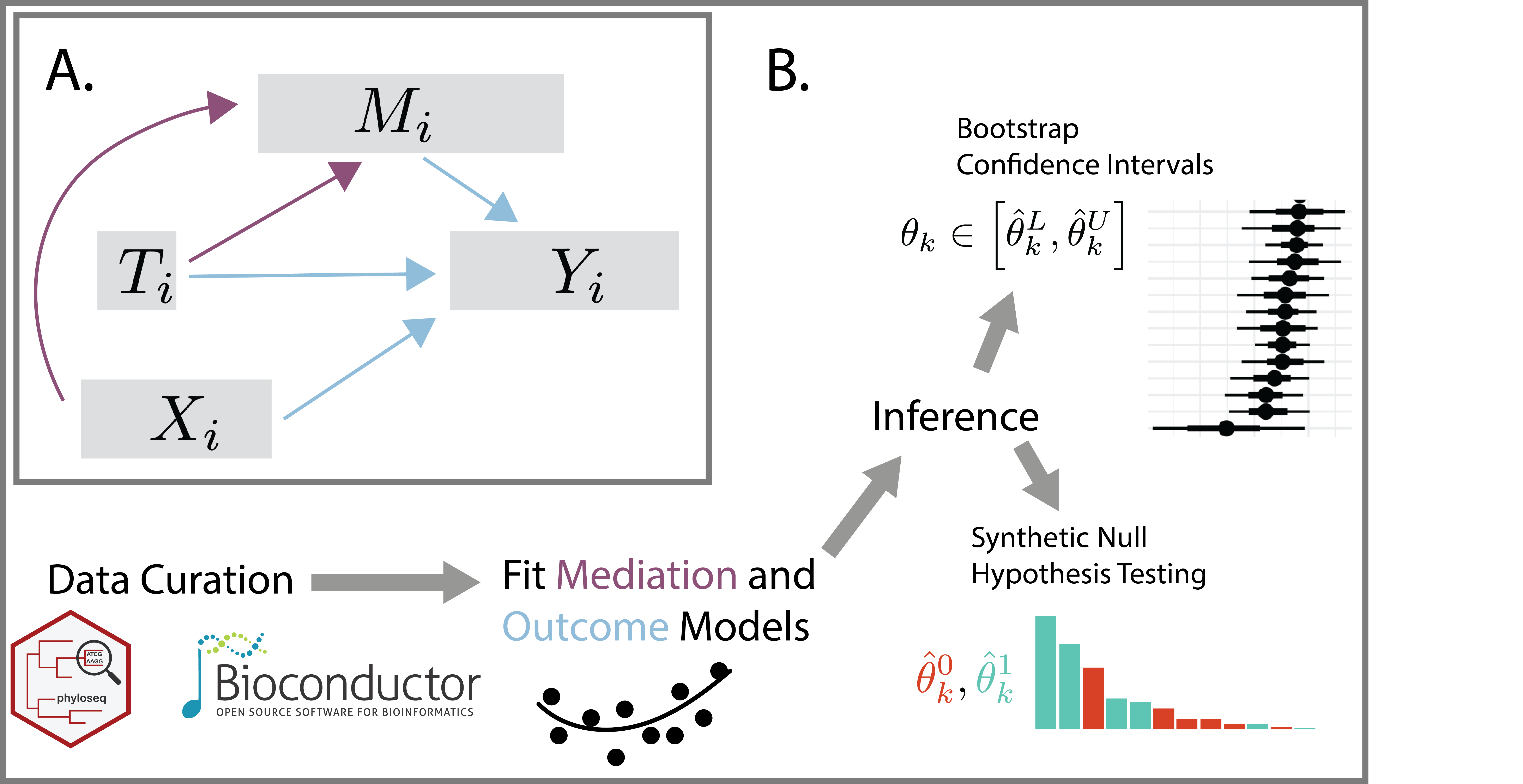

multimedia is an R package for
multimodal mediation analysis of
microbiome data. It streamlines data curation, mediation and outcome
model specification, and statistical inference for direct and indirect
effects. By defining causal relationships across data modalities, it can
support principled data integration. You can read more about the package
in our preprint:
The preprint describes the scientific context and interpretation for two of the vignettes in this package. One gives a multi-omics analysis of IBD, and the other describes how to simultaneously model 16S profiles and survey responses in a mindfulness intervention study.

You can install the development version from GitHub with:
# install.packages("devtools")
devtools::install_github("krisrs1128/multimedia")Here is a simple example of estimating direct and indirect effects.
The data are randomly generated (no real effects), but we imagine that
the ASV columns mediate the relationship between treatment
and PHQ. This is mimics the possibility that the microbiome
(ASV = Amplicon Sequence Variant) mediates the relationship between a
treatment and depression (PHQ = Patient Health Questionnaire). You can
find more details in the random.Rmd vignette.
The original data here are a SummarizedExperiment. The
package can also take phyloseq objects and data.frames.
library(multimedia)
demo_joy()
## class: SummarizedExperiment
## dim: 5 100
## metadata(0):
## assays(1): counts
## rownames(5): ASV1 ASV2 ASV3 ASV4 ASV5
## rowData names(0):
## colnames: NULL
## colData names(2): treatment PHQ
Next, we specify which columns are the treatment, mediators, and
outcomes. Notice that we can use tidyselect syntax to match
multiple columns.
exper <- mediation_data(demo_joy(), "PHQ", "treatment", starts_with("ASV"))
exper
## [Mediation Data]
## 100 samples with measurements for,
## 1 treatment: treatment
## 5 mediators: ASV1, ASV2, ...
## 1 outcome: PHQ
Next, we fit all mediation analysis components and estimate effects. By default, the package uses linear models – see the vignettes for examples using sparse regression, random forests, and bayesian hierarchical models instead.
model <- multimedia(exper) |>
    estimate(exper)
model
## [Multimedia Analysis]
## Treatments: treatment
## Outcomes: PHQ
## Mediators: ASV1, ASV2, ...
##
## [Models]
## mediation: A fitted lm_model().
## outcome: A fitted lm_model().
In any mediation analysis, there are several types of effects that
could be interesting, each corresponding to different ways of traveling
from the treatment to the outcome in the mediation analysis causal
graph. In the block below, direct_effect captures treatment
effects that bypass the microbiome; indirect_effect are
effects that are mediated by ASV relative abundances. Since this example
uses a linear model, the effects are identical for the two indirect
settings.
direct_effect(model, exper)## outcome indirect_setting
## 1 PHQ Control
## 2 PHQ Treatment
## contrast direct_effect
## 1 Control - Treatment 0.09314376
## 2 Control - Treatment 0.09314376
indirect_overall(model, exper)## outcome direct_setting contrast
## 1 PHQ Control Control - Treatment
## 2 PHQ Treatment Control - Treatment
## indirect_effect
## 1 0.02256029
## 2 0.02256029
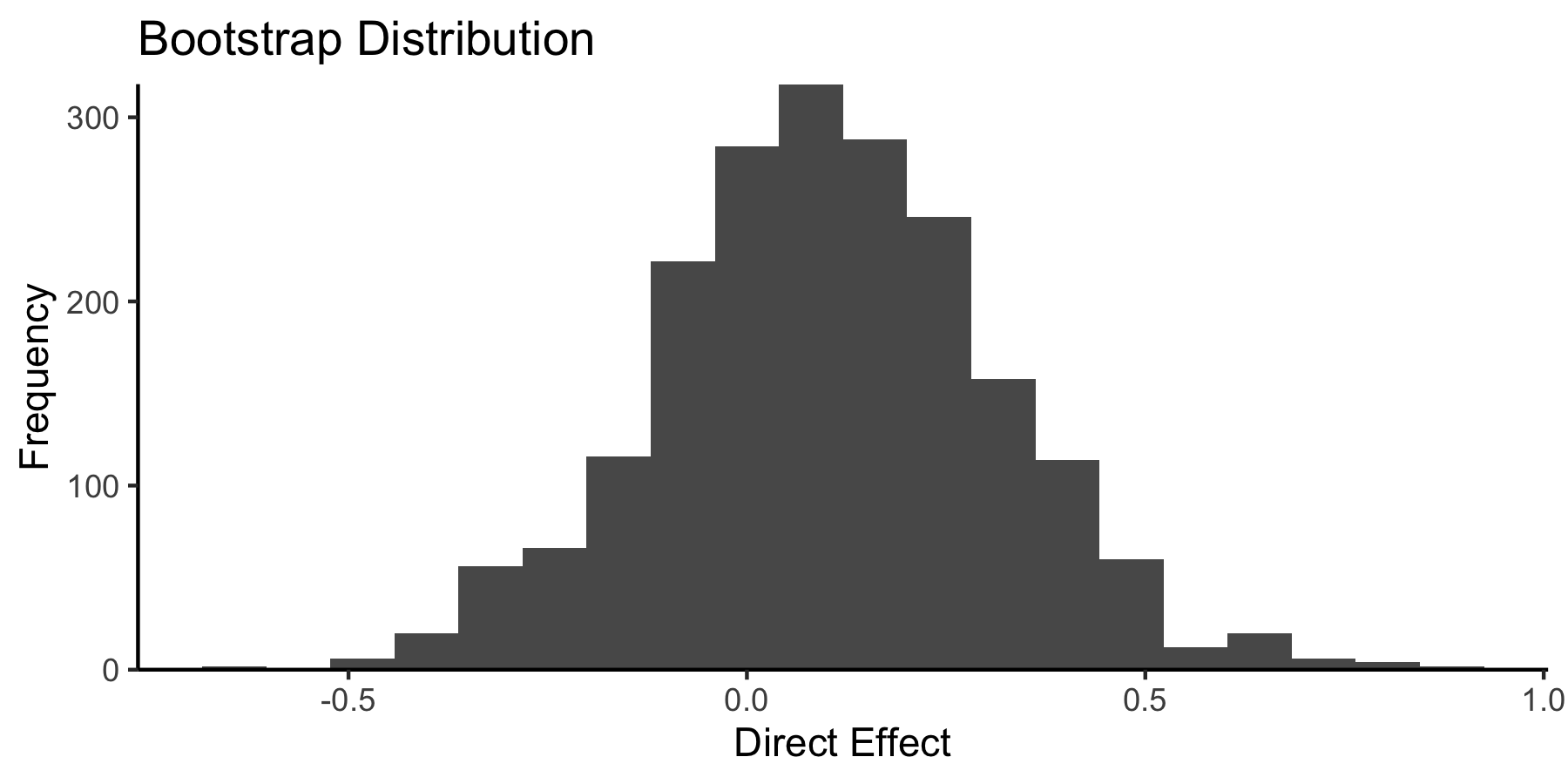
The package also includes helpers to visualize and perform inference on these effects. For example,
boot <- bootstrap(model, exper, c(direct = direct_effect))

library(ggplot2)
ggplot(boot$direct) +
    geom_histogram(aes(direct_effect), bins = 20) +
    scale_y_continuous(expand = c(0, 0)) +
    theme_classic() +
    labs(x = "Direct Effect", y = "Frequency", title = "Bootstrap Distribution")
If we want to use a different type of model, we can just modify the
original multimedia specification. Below we use a sparse
regression model, which correctly recovers that the direct effects are
0.
multimedia(exper, glmnet_model(lambda = .1)) |>
    estimate(exper) |>
    direct_effect()
## outcome indirect_setting
## 1 PHQ Control
## 2 PHQ Treatment
## contrast direct_effect
## 1 Control - Treatment 0
## 2 Control - Treatment 0
We welcome questions and comments about the package either through github or email.
sessionInfo()## R version 4.4.1 Patched (2024-08-21 r87049)
## Platform: aarch64-apple-darwin20
## Running under: macOS Sonoma 14.5
##
## Matrix products: default
## BLAS: /Library/Frameworks/R.framework/Versions/4.4-arm64/Resources/lib/libRblas.0.dylib
## LAPACK: /Library/Frameworks/R.framework/Versions/4.4-arm64/Resources/lib/libRlapack.dylib; LAPACK version 3.12.0
##
## locale:
## [1] en_US.UTF-8/en_US.UTF-8/en_US.UTF-8/C/en_US.UTF-8/en_US.UTF-8
##
## time zone: America/Chicago
## tzcode source: internal
##
## attached base packages:
## [1] stats graphics grDevices utils
## [5] datasets methods base
##
## other attached packages:
## [1] ggplot2_3.5.1 multimedia_0.2.0
## [3] tidyselect_1.2.1 ranger_0.16.0
## [5] glmnetUtils_1.1.9 brms_2.21.0
## [7] Rcpp_1.0.13
##
## loaded via a namespace (and not attached):
## [1] gridExtra_2.3
## [2] inline_0.3.19
## [3] permute_0.9-7
## [4] sandwich_3.1-0
## [5] rlang_1.1.4
## [6] magrittr_2.0.3
## [7] multcomp_1.4-26
## [8] ade4_1.7-22
## [9] matrixStats_1.4.1
## [10] compiler_4.4.1
## [11] mgcv_1.9-1
## [12] loo_2.8.0
## [13] vctrs_0.6.5
## [14] reshape2_1.4.4
## [15] stringr_1.5.1
## [16] pkgconfig_2.0.3
## [17] shape_1.4.6.1
## [18] crayon_1.5.3
## [19] fastmap_1.2.0
## [20] backports_1.5.0
## [21] XVector_0.45.0
## [22] labeling_0.4.3
## [23] utf8_1.2.4
## [24] rmarkdown_2.28
## [25] UCSC.utils_1.1.0
## [26] purrr_1.0.2
## [27] xfun_0.47
## [28] glmnet_4.1-8
## [29] zlibbioc_1.51.1
## [30] GenomeInfoDb_1.41.1
## [31] jsonlite_1.8.8
## [32] progress_1.2.3
## [33] biomformat_1.33.0
## [34] highr_0.11
## [35] rhdf5filters_1.17.0
## [36] DelayedArray_0.31.11
## [37] Rhdf5lib_1.27.0
## [38] prettyunits_1.2.0
## [39] cluster_2.1.6
## [40] parallel_4.4.1
## [41] R6_2.5.1
## [42] stringi_1.8.4
## [43] StanHeaders_2.32.10
## [44] GenomicRanges_1.57.1
## [45] estimability_1.5.1
## [46] rstan_2.32.6
## [47] SummarizedExperiment_1.35.1
## [48] iterators_1.0.14
## [49] knitr_1.48
## [50] zoo_1.8-12
## [51] IRanges_2.39.2
## [52] bayesplot_1.11.1
## [53] igraph_2.0.3
## [54] Matrix_1.7-0
## [55] splines_4.4.1
## [56] abind_1.4-5
## [57] yaml_2.3.10
## [58] vegan_2.6-8
## [59] codetools_0.2-20
## [60] curl_5.2.2
## [61] pkgbuild_1.4.4
## [62] lattice_0.22-6
## [63] tibble_3.2.1
## [64] plyr_1.8.9
## [65] withr_3.0.1
## [66] Biobase_2.65.1
## [67] bridgesampling_1.1-2
## [68] posterior_1.6.0
## [69] coda_0.19-4.1
## [70] evaluate_0.24.0
## [71] survival_3.7-0
## [72] RcppParallel_5.1.9
## [73] Biostrings_2.73.1
## [74] pillar_1.9.0
## [75] phyloseq_1.49.0
## [76] MatrixGenerics_1.17.0
## [77] tensorA_0.36.2.1
## [78] checkmate_2.3.2
## [79] foreach_1.5.2
## [80] stats4_4.4.1
## [81] distributional_0.4.0
## [82] generics_0.1.3
## [83] hms_1.1.3
## [84] S4Vectors_0.43.2
## [85] rstantools_2.4.0
## [86] munsell_0.5.1
## [87] scales_1.3.0
## [88] xtable_1.8-4
## [89] glue_1.7.0
## [90] emmeans_1.10.4
## [91] tools_4.4.1
## [92] data.table_1.16.0
## [93] mvtnorm_1.3-1
## [94] tidygraph_1.3.1
## [95] rhdf5_2.49.0
## [96] grid_4.4.1
## [97] tidyr_1.3.1
## [98] ape_5.8
## [99] QuickJSR_1.3.1
## [100] miniLNM_0.1.0
## [101] colorspace_2.1-1
## [102] nlme_3.1-166
## [103] formula.tools_1.7.1
## [104] GenomeInfoDbData_1.2.12
## [105] patchwork_1.2.0
## [106] cli_3.6.3
## [107] fansi_1.0.6
## [108] S4Arrays_1.5.7
## [109] Brobdingnag_1.2-9
## [110] dplyr_1.1.4
## [111] V8_5.0.0
## [112] gtable_0.3.5
## [113] digest_0.6.37
## [114] operator.tools_1.6.3
## [115] BiocGenerics_0.51.1
## [116] SparseArray_1.5.31
## [117] TH.data_1.1-2
## [118] farver_2.1.2
## [119] multtest_2.61.0
## [120] htmltools_0.5.8.1
## [121] lifecycle_1.0.4
## [122] httr_1.4.7
## [123] MASS_7.3-61